E-411 PRMA
Week 5 - Item Response Theory and Generalizability Theory
This Week
Item Response Theory
Generalizability Theory
Review
Classical Test Theory
X = T + E
\(\sigma^2_X = \sigma^2_T + \sigma^2_E\)
\(\sigma_{\text{SEM}} = \sigma \sqrt{1 - r_{xx}}\)
Critiques of CTT
- Person are measured on number correct
- Score dependent on number of items on a test and their difficulty
- Scores are limited to fixed values
- Scores are interpretable on a within-group normative basis
- SEM is group dependent and constant for a group
- Item and person fit evaluation difficult
- Test development different depending on type of test
Item Response Theory Rationale
In an nutshell, IRT is able to address all of these criticisms
BUT, makes stronger assumptions and requires a larger sample size
What is Item Response Theory?
A measurement perspective
A series of non-linear models
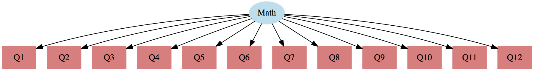
Links manifest variables with latent variables
Latent characteristics of individuals and items are predictors of observed responses
Not a "how" or "why" theory
Generalized Anxiety Disorder
Anxiety could be loosely defined as feelings that range from general uneasienss to incapcitating attacks of terror
Is anxiety latent and is it continuous, categorical, or both?
Categorical - Individuals can be placed into a high anxiety latent class and a low anxiety latent class
Continuous - Individuals fall along an anxiety continuum
Both - Given a latent class (e.g. the high anxiety latent class), within this class there is a continuum of even greater anxiety.
Properties of IRT
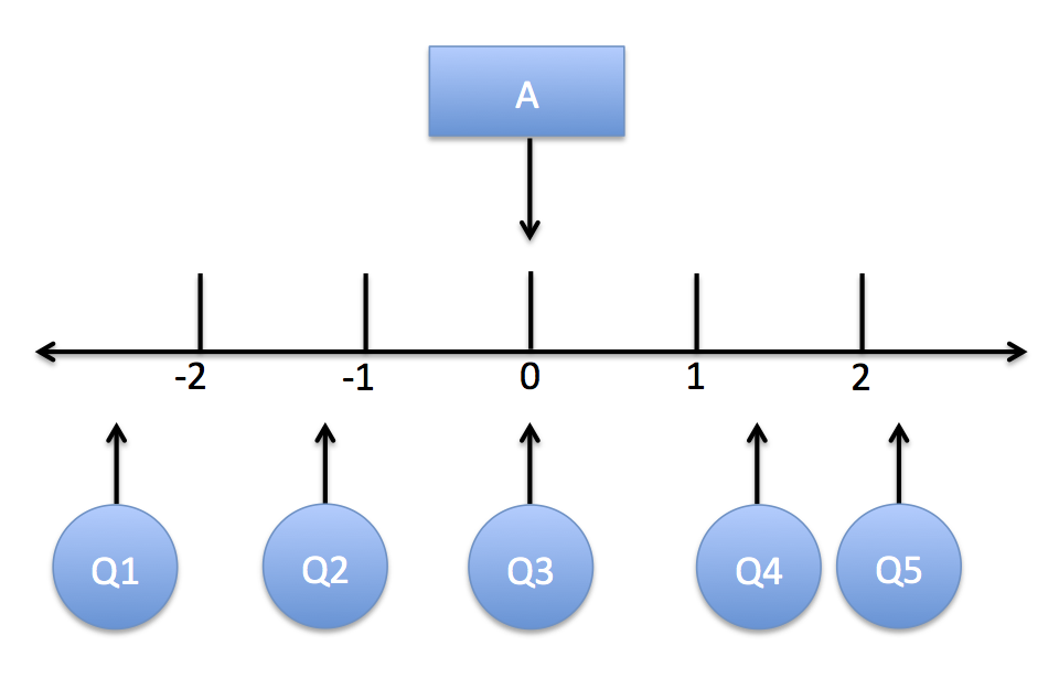
- Manifest variables differentiate among persons at different locations on the latent scale
- Items are characterized by location and ability to discriminate among persons
- Items and persons are on the same scale
- Parameters estimated in a sample are linearly transformable to estimates of those parameters from another sample
- Yields scores that are independent of number of items, item difficulty, and the individuals it is measured on, and are placed on a real-number scale
Assumptions of IRT
Response of a person to an item can be modeled with the a specific item reponse function
IRT conceptually
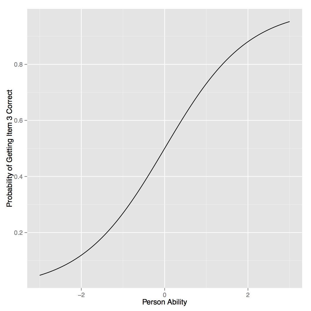
Item Response Function (IRF)
The Rasch Model
The logistic model
\(p(x = 1 | z) = \frac{e^z}{1 - e^z}\)
The logistic regression model
\(p(x = 1 | g) = \frac{e^{\beta_0 + \beta_1g}}{1 - e^{\beta_0 + \beta_1g}}\)
The Rasch model
\(p(x_j = 1 | \theta, b_j) = \frac{e^{\theta - b_j}}{1 - e^{\theta - b_j}}\)
So, the Rasch model is just the logistic regression model in disguise
What does \(\theta - b_j\) mean
rasch <- function(person, item) {
exp(person - item\) (1 + exp(person - item))
}
rasch(person = 1, item = 1.5)
# [1] 0.3775407

rasch(person = 1, item = 1)
# [1] 0.5
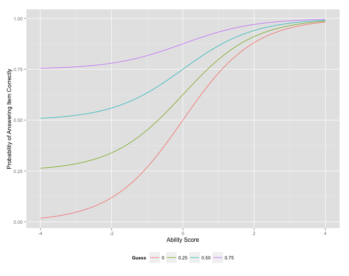
Guessing Parameter
Standard Error of Estimate and Information
Similar to the SEM, the standard error of estimate (SEE) allows us to quantify uncertainty about score of a person within IRT
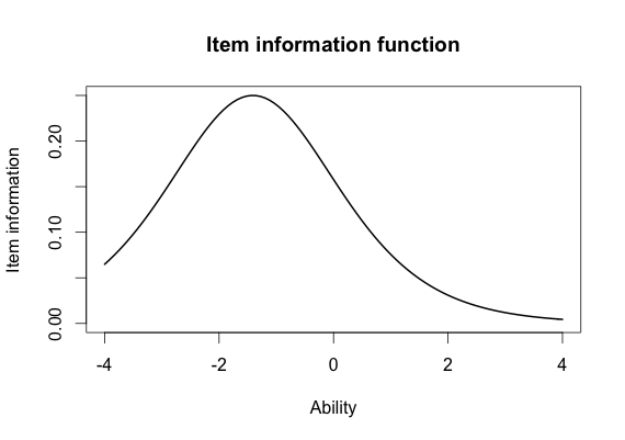
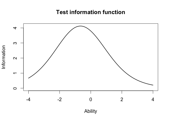
Information is the inverse of the SEE and tells us how precise our estimates
We can use this to select items and develop tests!
Item Information Function
Test Information Function
Generalizability Theory
Reliability is essentially a measure of consistency in your scores (think of a dart board)
Generalizability theory, the child of CTT, allows a researcher to quantify and distinguish the different sources of error in observed scores
The CTT model is: \(X = T + E\)
The G-Theory model is: \(X = \mu_p + E_1 + E_2 + \dots + E_H\)
\(\mu_p\) - universe score and \(E_h\) - are sources of error
G studies
- Suppose we develop a test to measure Icelandic writing abilities
- We have various items, people that will score the test (raters), and people that will take the test
- Item and rater are referred to as facets and any rater could rate any item (they are fully crossed)
- They could be considered fixed or random in a D study
- Universe are the conditions of measurement (item and rater) and population are the objects of measurement (people taking the test)
Our model
\(X_{pir} = \mu + v_p + v_i + v_r + v_{pi} + v_{pr} + v_{ir} + v_{pir}\)
If we assume that that these effects are uncorrelated then
\(\sigma^2(X_{pir}) = \sigma^2_p + \sigma^2_i + \sigma^2_r + \sigma^2_{pi} + \sigma^2_{pr} + \sigma^2_{ir} + \sigma^2_{pir}\)
These are our random effects variance components
This forms the basis of our D study which can investigate different scenarios and allow us to calculate reliability estimates
D study
In a D study, we partitition our variance into 3 components: universe score, relative error, and absolute error variance.
Relative error and the generalizability coefficient, are analagous to \(\sigma^2_E\) and reliability in CTT, and is based on comparing examinees
\(E\rho^2 = \frac{\sigma^2_\tau}{\sigma^2_\tau + \sigma^2_\delta}\)
Absolute error variance is for making absolute decisions about examinees
Dependability coefficient, \(\phi = \frac{\sigma^2_\tau}{\sigma^2_\tau + \sigma^2_\Delta}\)
Comparing G-Theory to CTT
- CTT reliability estimates are often too high
- Especially true when more than 1 random effect
- Different D-study scenarios allow you to investigate what-ifs based on treatment of effects, design, and number of subjects
- Universe score variance gets smaller if we consider a facet fixed instead of random
- Larger D study sample sizes lead to small error variances
- Nested D study designs usually lead to small error variances and larger coefficients